Where the sqrt(Δt) in a Wiener Process Comes From
The following was written by me, but reviewed by Claude for grammar and math mistakes.
While pure financial modeling may have limited edge in today’s world (machine learning is now the dominant source of edge feeding these models), it is still important – or at the very least, interesting – to know where these classical models came from. To start, there are a few prerequisite definitions. First off, it is important to note what a Markov process is– it is just a process where only the current value of a variable is relevant for predicting the future value. This assumption is generally used as a reflection of the weak form of market efficiency, which states that the present price of stocks contains all the information contained in a record of past prices. Evidently, this claim is very likely not true based on various papers12 and the existence of billion-dollar industries. Nonetheless, it is the first foundational assumption that all of the following work is built on.
Next, for another useful property: if the changes over two non-overlapping periods are independent and normally distributed, $X_1 \sim \mathcal{N}(\mu_1, \sigma_1^2)$ and $X_2 \sim \mathcal{N}(\mu_2, \sigma_2^2)$, then the total change over the combined period is distributed as
\[X_1 + X_2 \sim \mathcal{N}\left(\mu_1 + \mu_2,\ \sigma_1^2 + \sigma_2^2\right)\]That is, the means add and the variances add.
The Wiener process
Now, to get into the weeds of this article, we define a Wiener process as a particular type of Markov process with a mean change of zero and a variance rate of 1.0. Formally, it has the following properties:
Property 1: The change $\Delta z$ during a small period of time $\Delta t$ is
\[\Delta z = \epsilon \sqrt{\Delta t}\]where $\epsilon$ is a draw from a standardized normal distribution, $\epsilon \sim \mathcal{N}(0, 1)$.
Property 2: The values of $\Delta z$ for any two different short intervals of time, $\Delta t$, are independent.
As an immediate consequence of Property 1, we have:
- $E[\Delta z] = E\left[\epsilon \sqrt{\Delta t}\right] = \sqrt{\Delta t}\, E[\epsilon] = \sqrt{\Delta t} \cdot 0 = 0$, since $\sqrt{\Delta t}$ is a constant (so it factors out of the expectation by linearity) and $\epsilon \sim \mathcal{N}(0, 1)$ has mean zero
- $\text{Var}(\Delta z) = E\left[(\Delta z - E[\Delta z])^2\right] = E\left[\Delta z^2\right] = E\left[\epsilon^2 \Delta t\right] = \Delta t\, E\left[\epsilon^2\right] = \Delta t$
- $\text{SD}(\Delta z) = \sqrt{\text{Var}(\Delta z)} = \sqrt{\Delta t}$
where the second line starts from the definition of variance and uses the fact that $\Delta t$ is a constant along with the second moment of the standard normal, $E\left[\epsilon^2\right] = \text{Var}(\epsilon) + E[\epsilon]^2 = 1 + 0 = 1$.
Moreover, Property 2 immediately tells us that a Wiener process is Markov.
(For a cool related fact – the expected length of the path followed by $z$ in any time interval is infinite – see the appendix.)
Generalizing it
Now, to generalize Wiener for a variable $x$:
\[dx = a\,dt + b\,dz\]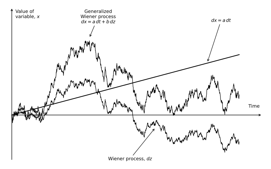
Figure adapted from Options, Futures, and Other Derivatives.3
Here, $b\,dz$ is considered the “noise” term. If it were zero, we’d have a very well defined $dx = a\,dt$ and could immediately solve to get $x = x_0 + at$. Moreover, a Wiener process has a variance rate per unit time of 1.0. It follows, since variance scales quadratically, that “$b$ times a Wiener process” has a variance rate per unit time of $b^2$ (remember, we interpret models in terms of standard deviation but we use variance because it is algebraically simpler to work with). So, in a generalized Wiener process, Property 1 becomes
\[\Delta x = a\,\Delta t + b \epsilon \sqrt{\Delta t}\]Repeating the same derivation as before:
- $E[\Delta x] = a\,\Delta t + b \sqrt{\Delta t}\, E[\epsilon] = a\,\Delta t$
- $\text{Var}(\Delta x) = E\left[(\Delta x - E[\Delta x])^2\right] = E\left[b^2 \epsilon^2 \Delta t\right] = b^2\, \Delta t\, E\left[\epsilon^2\right] = b^2\, \Delta t$
- $\text{SD}(\Delta x) = b \sqrt{\Delta t}$
where the variance line also uses that deterministic shifts don’t move variance: the drift term $a\,\Delta t$ is a constant, so only the noise term survives $\Delta x - E[\Delta x]$.
Moreover, over a general $T$ (not a small $\Delta t$), we have
\[x(T) - x(0) \sim \mathcal{N}\left(aT,\ b^2 T\right)\]To see this, split $[0, T]$ into $N = T / \Delta t$ small intervals. By Property 2, the increments $\Delta x_i$ are independent, so by the additivity property from earlier, the means and the variances of the $N$ increments add:
- $E[x(T) - x(0)] = \sum_{i=1}^{N} E[\Delta x_i] = N \cdot a\,\Delta t = aT$
- $\text{Var}(x(T) - x(0)) = \sum_{i=1}^{N} \text{Var}(\Delta x_i) = N \cdot b^2\,\Delta t = b^2 T$
and a sum of independent normal variables is itself normal. The standard deviation of $x(T) - x(0)$ is therefore $b \sqrt{T}$: uncertainty grows with the square root of elapsed time.
Why sqrt(Δt)?
Now, for the goal of this post: why $\sqrt{\Delta t}$? Why not just have
\[\Delta x = a\,\Delta t + b \epsilon\, \Delta t\]Let’s explore the consequences of that:
If we did that, we’d now have a per-step variance of
\[\text{Var}(\Delta x) = E\left[(\Delta x - E[\Delta x])^2\right] = E\left[b^2 \epsilon^2 \Delta t^2\right] = b^2\, \Delta t^2\, E\left[\epsilon^2\right] = b^2\, \Delta t^2\]by exactly the same steps as before.
This would lead to an overall variance over a period $T$ (again splitting it into $N = T / \Delta t$ independent increments whose variances add) of
\[\text{Var}(x(T) - x(0)) = N \cdot b^2\, \Delta t^2 = \frac{T}{\Delta t} \cdot b^2\, \Delta t^2 = b^2\, T\, \Delta t\]which would go to zero as $\Delta t$ goes to zero! That is to say, we would be able to predict exactly the terminal value of this process and nothing is very interesting– we would just have a straight line.
Ok, but what if we do some other power? What about the fourth root of $\Delta t$? In general, let’s take a look at
\[\Delta x = a\,\Delta t + b \epsilon\, (\Delta t)^p\]where $p \in \mathbb{R}^+$. This would give us a per-step variance of
\[\text{Var}(\Delta x) = E\left[b^2 \epsilon^2 (\Delta t)^{2p}\right] = b^2\, (\Delta t)^{2p}\, E\left[\epsilon^2\right] = b^2\, (\Delta t)^{2p}\]which would give us a total variance over a period $T$ of
\[\text{Var}(x(T) - x(0)) = N \cdot b^2\, (\Delta t)^{2p} = \frac{T}{\Delta t} \cdot b^2\, (\Delta t)^{2p} = b^2\, T\, (\Delta t)^{2p - 1}\]Now everything hinges on the exponent $2p - 1$:
- If $p > 1/2$, then $(\Delta t)^{2p - 1} \to 0$ as $\Delta t \to 0$: the variance vanishes and we are back to a deterministic straight line.
- If $p < 1/2$, then $(\Delta t)^{2p - 1} \to \infty$ as $\Delta t \to 0$: the variance blows up over any finite interval.
- Only $p = 1/2$ makes the exponent exactly zero, leaving $\text{Var}(x(T) - x(0)) = b^2\, T$: finite, nonzero, and independent of how finely we slice the interval.
That is, the only reasonable, interesting value here is $p = 1/2$. Hence why the square root makes its way in. We could probably use non-polynomial functions but that would just complicate future work. $\sqrt{\Delta t}$ is the simplest we can get here.
Appendix: Simulate it yourself
The whole construction is just Property 1 applied $N$ times and accumulated with a cumulative sum – a few lines of NumPy. Seed 14 reproduces the exact paths in the figure above; change the seed, $a$, or $b$ and see what happens:
import numpy as np
import matplotlib.pyplot as plt

a, b = 0.3, 1.5
T, N = 25.0, 1500
dt = T / N

t = np.linspace(0, T, N + 1)
eps = np.random.default_rng(seed=14).standard_normal(N)

z = np.concatenate([[0.0], np.cumsum(eps * np.sqrt(dt))])
x = a * t + b * z

plt.plot(t, a * t, label=r"$dx = a\,dt$ (drift only)")
plt.plot(t, x, label=r"$dx = a\,dt + b\,dz$ (generalized Wiener)")
plt.plot(t, z, label=r"Wiener process, $z$")
plt.xlabel("Time")
plt.ylabel(r"Value of variable, $x$")
plt.legend()
plt.show()
To see the point of this post in action, replace np.sqrt(dt) with dt ** p: for $p > 1/2$ the noise flattens out and the path hugs the drift line, and for $p < 1/2$ it swamps everything. Crank $N$ up while you’re at it – only $p = 1/2$ keeps the picture stable as the steps get finer.
Or play with it right here, no Python required. The random shocks $\epsilon_i$ are held fixed while you move the slider, so what you are watching is purely the effect of $p$; hit the button for a fresh set of shocks. The readout under the chart tracks the total variance $b^2\, T\, (\Delta t)^{2p - 1}$ from the derivation above:
Appendix: The Probability Toolbox
For reference, here is every statistics and probability fact the derivations above leaned on, and where each one did its work:
-
Linearity of expectation: $E[X + Y] = E[X] + E[Y]$ and $E[cX] = c\,E[X]$ for any constant $c$ – no independence assumption required. Used to pull $\sqrt{\Delta t}$ out of $E[\Delta z]$, to split $E[\Delta x]$ into its drift and noise pieces, and to turn $E[x(T) - x(0)]$ into a sum of the $N$ per-interval means.
-
Mean of the standard normal: $E[\epsilon] = 0$ for $\epsilon \sim \mathcal{N}(0, 1)$. This is what kills the noise term in both $E[\Delta z] = 0$ and $E[\Delta x] = a\,\Delta t$.
-
Definition of variance: $\text{Var}(X) = E\left[(X - E[X])^2\right]$. The starting point of both variance computations.
-
Second moment of the standard normal: $E[\epsilon^2] = \text{Var}(\epsilon) + E[\epsilon]^2 = 1$. This is the shortcut formula $\text{Var}(X) = E[X^2] - E[X]^2$ run in reverse; it converts $E[\epsilon^2 \Delta t]$ into $\Delta t$ in both variance bullets.
-
Deterministic shifts don’t move variance: $\text{Var}(X + c) = \text{Var}(X)$. Used implicitly in $\text{Var}(\Delta x)$: the drift term $a\,\Delta t$ is deterministic, so only the noise term $b \epsilon \sqrt{\Delta t}$ contributes.
-
Scaling is linear in expectation but quadratic in variance: $\text{Var}(cX) = c^2\,\text{Var}(X)$. This is why “$b$ times a Wiener process” has a variance rate of $b^2$, and – taking the square root back out – why every standard deviation in this post ends up under a radical.
-
Variances add under independence: $\text{Var}(X + Y) = \text{Var}(X) + \text{Var}(Y) + 2\,\text{Cov}(X, Y)$, and the covariance term vanishes for independent variables. This is the one place independence (Property 2) is truly load-bearing: it lets the $N$ per-interval variances sum to $b^2 T$ in the $x(T) - x(0)$ proof. Contrast with expectations, which add unconditionally.
-
Sums of independent normals are normal: the normal family is closed under independent addition. This upgrades “mean $aT$, variance $b^2 T$” to the full distributional statement $x(T) - x(0) \sim \mathcal{N}\left(aT,\ b^2 T\right)$.
-
Mean absolute value of the standard normal: $E\lvert\epsilon\rvert = \sqrt{2/\pi} \approx 0.798$ – the mean of the half-normal distribution. Without doing the full work, here is the integral it comes from:
\[E\left|\epsilon\right| = \int_{-\infty}^{\infty} \lvert x \rvert\, \frac{e^{-x^2/2}}{\sqrt{2\pi}}\, dx = \frac{2}{\sqrt{2\pi}} \int_{0}^{\infty} x\, e^{-x^2/2}\, dx = \frac{2}{\sqrt{2\pi}} \cdot 1 = \sqrt{\frac{2}{\pi}}\]The density is symmetric, so integrating $\lvert x \rvert$ is twice the positive half; then the substitution $u = x^2/2$ turns the remaining integral into $\int_0^\infty e^{-u}\, du = 1$. (The $\pi$ is hiding in the density’s normalizing constant $\sqrt{2\pi}$ – that one is the famous change-of-coordinates trick, where you square the Gaussian integral and switch to polar coordinates.) Used in the path-length appendix to compute the expected size of a single step, $E\lvert\Delta z\rvert$.
Appendix: The expected path length of a Wiener process is infinite
This is a cool fact that I could not resist writing about, but that I also don’t want to give a full blog post. Going back to a simple Wiener (not generalized):
\[\Delta z = \epsilon \sqrt{\Delta t}\]What is the sum of this path over any period $T$?
The distance the path travels is the sum of the absolute values of its steps. Splitting $[0, T]$ into $N = T / \Delta t$ steps as usual, the path length is
\[L = \sum_{i=1}^{N} \left|\Delta z_i\right| = \sum_{i=1}^{N} \left|\epsilon_i\right| \sqrt{\Delta t}\]Taking expectations, by linearity and the mean absolute value of the standard normal, $E\lvert\epsilon\rvert = \sqrt{2/\pi}$:
\[E[L] = N \cdot \sqrt{\frac{2}{\pi}}\, \sqrt{\Delta t} = \frac{T}{\Delta t} \cdot \sqrt{\frac{2}{\pi}}\, \sqrt{\Delta t} = \sqrt{\frac{2}{\pi}}\, \frac{T}{\sqrt{\Delta t}}\]which goes to infinity as $\Delta t \to 0$. So over any interval, no matter how short, the expected distance traveled by a Wiener process is infinite – even though it only ends up on the order of $\sqrt{T}$ away from where it started. (In the language of analysis: Wiener paths have unbounded variation.)
Does this survive the generalization $\Delta x = a\,\Delta t + b \epsilon \sqrt{\Delta t}$? Yes, whenever $b \neq 0$. Per step, the drift contributes order $\Delta t$ while the noise contributes order $\sqrt{\Delta t}$, so at small scales the noise dominates every step. Using the reverse triangle inequality, $\lvert X + c \rvert \geq \lvert X \rvert - \lvert c \rvert$:
\[E[L] = \sum_{i=1}^{N} E\left|a\,\Delta t + b \epsilon_i \sqrt{\Delta t}\right| \geq \frac{T}{\Delta t} \left( \lvert b \rvert \sqrt{\frac{2}{\pi}}\, \sqrt{\Delta t} - \lvert a \rvert\, \Delta t \right) = \sqrt{\frac{2}{\pi}}\, \frac{\lvert b \rvert\, T}{\sqrt{\Delta t}} - \lvert a \rvert\, T\]which still goes to infinity as $\Delta t \to 0$. The drift can only ever contribute $\lvert a \rvert\, T$ of length in total – a straight line’s worth – while the noise contributes on the order of $T / \sqrt{\Delta t}$. Only the degenerate case $b = 0$ has a finite expected path length.
Appendix: What breaks without Property 2
Property 2 – independent increments – is an assumption, and everything in this post leans on it. (It is not the same as the Markov property: a mean-reverting process is perfectly Markov, yet its increments are correlated.) If we drop it:
What survives. Anything built on linearity of expectation, which holds unconditionally: the per-step facts, and the drift $E[x(T) - x(0)] = aT$.
What breaks. Variances add only when the covariances vanish. In general,
\[\text{Var}\left( \sum_{i=1}^{N} \Delta x_i \right) = \sum_{i=1}^{N} \text{Var}(\Delta x_i) + 2 \sum_{i < j} \text{Cov}(\Delta x_i, \Delta x_j)\]Independence is what killed the second sum, and it has roughly $N^2/2$ terms against the first sum’s $N$.
// TODO: write another blog post to explore this more.
Appendix: Sources
-
Andrew W. Lo and A. Craig MacKinlay, “Stock Market Prices Do Not Follow Random Walks: Evidence from a Simple Specification Test”, The Review of Financial Studies, Vol. 1, No. 1, 1988, pp. 41-66. ↩
-
Mikio Ito and Shunsuke Sugiyama, “Measuring the degree of time varying market inefficiency”, Economics Letters, Vol. 103, No. 1, 2009, pp. 62-64. ↩
-
John C. Hull, Options, Futures, and Other Derivatives, Global Edition, 11th ed., Pearson, Figure 13.2, page 321. ↩